Interference in Phased Array and Conservation of Energy
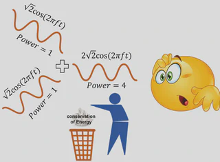
Have you ever come across a question that seems simple at first glance but lingers in your mind, challenging your understanding of fundamental principles? One such brain teaser that often puzzles students of electromagnetic (EM) waves or antenna theory is the behavior of power when coherent sources interfere. The figure below illustrates this intriguing scenario.
The law of conservation of energy is a cornerstone of physics, holding true in every known phenomenon. So, if the argument in the figure appears to defy this law, there must be a flaw in the reasoning. This post tackles this question from two angles: first, by examining what happens to energy during constructive and destructive interference of individual EM waves, and second, by exploring the behavior of radiated power in systems with multiple phased antennas.
Problem description of an apparent paradox
Let’s formally present the paradox shown in the figure. Imagine case 1: we have a sinusoidal signal $x_1(t) = A\sin(2\pi f_c t)$, and its power is calculated using the formula commonly found in signal theory books:
$${\rm Power} = \frac{1}{T}\int_{0}^{T} \vert x(t) \vert^2 dt$$Here, $A$ is the amplitude, and $T$ is the time period of the signal $x(t)$. Using this, the power of $x_1(t)$ is $P_1 = A^2/2$ units. Now, consider case 2: two identical signals combine constructively. By the superposition principle, $x_2(t) = 2x_1(t) = 2A\sin(2\pi f_c t)$. Calculating the power, we find $P_2 = 4A^2/2 = 4P_1$ units. But wait—if the total power of the individual signals is only $2P_1$, where did the extra $2P_1$ come from? This puzzling question gives rise to the paradox and the apparent violation of energy conservation.
Short Answer:
- If the setup involves wires, such a situation is physically impossible.
- In a phased array, the received power is always less than the radiated power.
- For two EM waves traveling in opposite directions, energy is conserved because when electric energy doubles, magnetic energy drops to zero, and vice versa. The total energy, being the sum of electric and magnetic field energies, remains constant.
The mathematical justification for these points follows next.
Equivalent circuit for the above phenomenon
Let’s start with a counterargument: it’s impossible to create a circuit that produces the paradox described earlier. And if it’s impossible in a wired circuit, it’s even more unlikely in a wireless setup. Let’s examine two cases similar to the earlier discussion.
Case 1: Consider an AC circuit with a voltage source $V_1(t) = A\sin(\omega_c t)$ (in volts), as shown below:

Network 1
The AC current in this circuit is $I_1(t) = A\sin(\omega_c t)$ (in amperes). The average power dissipated across the resistor is:
$$P_1 = \frac{1}{T}\int_{0}^{T} V_1(t)^2 dt$$This results in $P_1 = A^2/2$ W. The power delivered by the voltage source is:
$$P_{s1} = \frac{1}{T}\int_{0}^{T} V_1(t)I_1(t) dt$$which also gives $P_{s1} = A^2/2$ W. So far, so good.
Case 2: Now consider two voltage sources connected in series, as shown below:

Network 2
The total voltage across the resistor is $V_2(t) = 2A\sin(\omega_c t)$ V. The total power dissipated across the resistor is:
$$P_2 = \frac{1}{T}\int_{0}^{T} V_2(t)^2 dt$$This gives $P_2 = 4A^2/2$ W, matching the claim in the paradox. However, the power delivered by each source, $P_{s1}$ and $P_{s2}$, is not $A^2/2$ W as in the individual case. Instead, the power delivered by each source is:
$$P_{s1} = P_{s2} = \frac{1}{T}\int_{0}^{T} V_1(t)I_2(t) dt$$where $I_2(t) = 2A\sin(\omega_c t) = 2I_1(t)$. In other words, when connected in series with another voltage source (with zero phase difference), each source delivers more current than when operating alone. From the calculations, $P_{s1} = P_{s2} = 2A^2/2$ W. Thus, each voltage source delivers twice the power it would when operating alone. The law of energy conservation holds.
Key takeaway: The power delivered by sources isn’t always proportional to the square of voltage or current. It’s safer to calculate the product of voltage and current, especially when multiple sources are involved. In the example above, the voltage and current amplitudes differ, leading to the observed results.
Disclaimer: further reading is intended for readers who are interested to know how interference behaves in wireless communication. Some fundamental background in EM and basic antenna theory is expected.
Phased Antenna Array
Let’s now explore how multiple antenna elements radiate together. We’ll consider two cases: one with a single source and another with two sources. For simplicity, we’ll use isotropic antennas—idealized references that don’t exist in reality but are handy for explanations.
Case 1: A single isotropic source. The electric field of an isotropic antenna in the far field at a reference distance $r$, in terms of elevation angle $\theta$ and azimuthal angle $\phi$, is given by $E_1(\theta,\phi) = \frac{E_0}{r}$. The magnetic field at the same reference distance is $H_1$. The time-averaged Poynting vector is:
$$ \begin{align} S(\theta,\phi) &= \frac{1}{2}\Re\{E_1\times H_1^{*}\}\\ &=\frac{1}{2Z_0}\vert E_1 (\theta,\phi) \vert^2\quad[{\rm W/m^2}] \end{align} $$Here, $H_1$ is the magnetic field at the reference distance, and $Z_0$ is the intrinsic impedance of free space. In the far field, $\vert E_1\vert/\vert H_1\vert = Z_0$. The radiation intensity, $U(\theta,\phi)$, is:
$$U(\theta,\phi) = r^2S(\theta,\phi)\quad[{\rm W/sr}]$$This represents the angular distribution of time-averaged power, also denoted as $\partial P(\theta,\phi)/\partial \Omega$. The total radiated power is:
$$ \begin{align} P_1 &= \int_{0}^{2\pi}\int_{0}^{\pi}U(\theta,\phi)\sin(\theta,\phi)d\theta d\phi\\ &=\frac{1}{2Z_0}\vert E_0 \vert^2 4\pi\\ &=12.56 A_1^2\quad [{\rm W}] \end{align} $$where $A_1^2 = \frac{1}{2Z_0}\vert E_0 \vert^2$.
Case 2: Two isotropic sources placed on the y-axis at $(0,-\frac{\Delta}{2},0)$ and $(0,\frac{\Delta}{2},0)$. The observing reference is in the far field and in the direction $\bar{n} = (\sin(\theta)\cos(\phi),\sin(\theta)\sin(\phi),\cos(\theta))$. The approximate path length difference between the wave traveling from these two sources is $\bar{n}\cdot \bar{d}$, where $\bar{d} = (0,\Delta,0)$.
With the above assumptions, the total phase difference between the waves in the far field is
$$ \psi = \frac{2\pi}{\lambda} \bar{n}\cdot \bar{d} + \psi_0 $$where $\psi_0$ is the initial phase difference between the sources. From the principle of superposition, the total electric field is
$$ \begin{align} E_2 &= E_1 + E_1e^{i\psi}\\ &= 2E_1e^{i\frac{\psi}{2}}\cos\left(\frac{\psi}{2}\right) \end{align} $$The effective radiation intensity is then given by (Note: if below equations are not rendering properly in mobile browser then in browser options select “desktop site”)
$$ \begin{align} U_2(\theta,\phi) &= \frac{r^2}{2Z_0}\vert E_2 \vert^2\\ &=\frac{1}{2Z_0}4\vert E_0 \vert^2 \cos^2\left(\frac{\pi}{\lambda}\bar{n}\cdot\bar{d} + \frac{\psi_0}{2}\right)\\ &=4A_1^2 \left[\cos^2\left(\frac{\psi_0}{2}\right)\cos^2 \left(\frac{\pi\Delta}{\lambda} \sin(\theta)\sin(\phi)\right)\right.\\ &\qquad + \sin^2\left(\frac{\psi_0}{2}\right)\sin^2 \left(\frac{\pi\Delta}{\lambda} \sin(\theta)\sin(\phi)\right)\\ &\qquad -\left.\frac{1}{2}\sin\left(\psi_0\right)\sin\left(\frac{2\pi\Delta}{\lambda}\sin(\theta)\sin(\phi)\right)\right] \end{align} $$The total radiated power is
$$ P_2 = \int_{0}^{2\pi}\int_{0}^{\pi}U_2(\theta,\phi)\sin(\theta) d\theta d\phi $$Now we present three different situations and give an interpretation behind them:
Case 2a: $\Delta = \frac{\lambda}{2}$ and $\psi_0 = \frac{\pi}{2}$
$$ \begin{align} P_2 &= 4A_1^2 \int_{0}^{2\pi}\int_{0}^{\pi} \cos^2\left(\frac{\pi}{4}\sin(\theta)\sin(\phi)\right) \sin(\theta) d\theta d\phi \\ &= 8\pi A_1^2 \\ &= 2P_1 \end{align} $$So, in this case, the total radiated power equals the sum of radiated powers of individual sources. In this case, we say there is no mutual coupling between antennas.
So, in this case, the total radiated power equals the sum of radiated powers of individual sources. In this case, we say there is no mutual coupling between antennas.
Then one may wonder what is the benefit of having two antennas. The answer lies in the observation that in the case of practical wireless systems, the power is radiated outwards like a balloon but is not pointed as a sharp laser beam. So first consider the total radiated power in both cases (single source and two sources) to be same, i.e. let the total power radiated in a single antenna case be $2P_1$ then let us consider the direction in which the radiation intensity (or average power per solid angle) is maximum, and this happens in any direction for the case of a single source (since it is isotropic) and for the case of two sources $\theta = \frac{\pi}{2}, \phi = -\frac{\phi}{2}$ (one of the case) and is given as
$$ \begin{align} \left(\frac{\partial P_2(\theta,\phi)}{\partial \Omega}\right)_{\rm max} &= 4A_1^2 \\ &= 2 \cdot 2\left(\frac{\partial P_1(\theta,\phi)}{\partial \Omega}\right)_{\rm max} \\ &\approx 0.16 P_2 \end{align} $$Thus, we can see that in the most favourable direction, the power gain with two isotropic antennas is $2$ compared to a single isotropic antenna source. This is called beamforming gain or array power gain. What we mean by beamforming gain of 2 for two elements isotropic antenna array is that we receive $2$ times more power when compared to a single source case. In other words, to receive the same power in two cases, two antenna (isotropic) systems need half the power as that of a single source (isotropic) case. However, the fraction of power that is received is $\left(\frac{\partial P_2(\theta,\phi)}{\partial \Omega}\right)_{\rm max} \approx 0.16 P_2$ which is still very less than total radiated power. Thus, in wireless as well, there is no paradox.
Similar to the single antenna case, we can write the fraction of power received at the isotropic antenna that is placed in the most favourable direction
$$\partial P_2\left(\frac{\pi}{2},-\frac{\pi}{2}\right) = 2\beta P_2 = 4\beta P_1$$As such, this case may sometimes lead to an incorrect impression that received power is a fraction of $4 P_1$. What is actually happening is that in the case of two isotropic antennas, the power pattern is not uniformly distributed on a sphere as was the case with a single antenna source. Rather, it is dumbbell-shaped, and power is just redistributed. In simple words, if we have $2 P_1$ power in the case of a single antenna case (these to make fare comparison between two cases in terms of radiated power), then all the points on the sphere would receive $\beta 2P_1$ power and now if we remove the power from half of the points on that sphere and redistribute it uniformly in other places then we would have two regions with received powers as $\beta 2P_1 + \beta 2P_1 = \beta 4P_1$ and $\beta 2P_1 - \beta 2P_1 =0$, respectively. These respective regions are locations of constructive and destructive interference.
Case 2b: $\Delta = \frac{\lambda}{4}$ and $\psi_0 = 0$
$$ \begin{align} P_2 &= 4A_1^2\int_{0}^{2\pi}\int_{0}^{\pi}\cos^2\left(\frac{\pi}{4}\sin(\theta)\sin(\phi)\right) d\theta d\phi \\ & \approx 3.27 (4\pi)A_1^2 \\ &= 3.27P_1 \end{align} $$In this case, the total radiated power is larger than the sum of radiated powers of individual sources when acting alone. In this case, we say there is positive mutual coupling between antennas. What is happening is that the radiation of one antenna is influencing the other antenna and overall changing the impedance seen by the two sources, which in turn affects the radiated power. More specifically, in this case, the radiated power by at least one of the antenna source is larger than $P_1$, i.e. the antenna is radiating more power than it was acting alone. To know more precisely how much each antenna radiates depends on the phases of the exicitation currents of the sources and mutual impedences and these concepts are beyond the intended aim of this article.
If in case the total input drive power is just $2P_1$ then we need to renormalize $U_2(\theta,\phi)$ by $2/3.27$ and if the total drive power is $P_1$ then the renormalizing factor is $1/3.27$. In this case, $\left(\frac{\partial P_2(\theta,\phi)}{\partial \Omega}\right)_{\rm max} \approx 1.22 \left(\frac{\partial P_1(\theta,\phi)}{\partial \Omega}\right)_{\rm max}$ and hence the beamforming gain is 1.22. Thus, it shows if there is coupling between the antennas, then there is a significant reduction in the beamforming gain [1], [5]. In the most extreme case, if $\Delta \approx 0$, the total radiated power is four times the single antenna case. This case resembles the same situation as that of the circuit example presented previously, and in principle, each antenna radiates twice the power than it was radiating when acting alone [3-4]. Also, to add if we introduce phase difference in the circuit example, we can produce these three cases in a circuit as well. Thus, the circuit example can be thought of as maximum positive coupling among the sources.
This case of mutual coupling may sometimes lead to the misimpression that the received power can be computed without renormalization and that more power is radiated than the total drive power.
Case 2c: $\Delta = \frac{\lambda}{4}$ and $\psi_0 = \pi$
$$ \begin{align} P_2 &= \int_{0}^{2\pi}\int_{0}^{\pi}\cos^2\left(\frac{\pi}{4}\sin(\theta)\sin(\phi)+ \frac{\pi}{2}\right),d\theta ,d\phi\\ & \approx 0.73 (4\pi)A_1^2\\ &= 0.73P_1 \end{align} $$In this case, the total radiated power is much less than the source acting alone. This is said due to the fact that the effective impedance seen by the antenna array is very high, and hence radiated power is reduced. In the most extreme case, if $\Delta \approx 0$, then total radiated power is zero, and this can be thought of as a global destructive interference because, at each point in space, the net electric field is zero. However, this doesn’t violate any energy conservation law because the power doesn’t radiate at all and is within the system itself because the effective impedance seen by the antenna array approaches infinity.
So, in general, with two sources, total radiated power can be written as
$$P_{\rm total} = P_1 + P_2 + P_{\rm coupling}$$where $P_1$ and $P_2$ is the power radiated by two sources and $P_{\rm coupling}$ is the coupling power which can be negative, zero and positive. So in most cases $-(P_1+P_2)\leq P_{\rm coupling} \leq P_1+P_2$. Negative coupling doesn’t mean power is lost but should be interpreted as the power didn’t radiate from antennas. Such examples can also be produced by adjusting the phase difference in wired circuits and studying how power drawn from each source behave.
If you are interested, then you can use the below MATLAB code snippet to play around with $\Delta$ and $\psi_0$ and see how radiated power varies:
% Antenna array spacing and initial phase difference
delta_lambda = 0.25; % Delta/Lambda
psi_0 = pi;

% Radiation intensity
U = @(x,y)4*sin(x).*(cos(psi_0/2 + pi*delta_lambda*sin(x).*sin(y))).^2;

% Radiated power
Prad = integral2(U,0,pi,0,2*pi);

% Factor of radiated power compared to single isotropic antenna
factor = Prad/(4*pi);
The channel gain and beamforming gains presented were only for identically excited isotropic antenna elements. However, these values depend on the antenna type, spacing between them, initial phase difference and also on excitation of antenna elements. So an interesting question to ponder is how large can the array power gain be, or is there any upper bound?
Constructive/Destructive interference with EM waves
There’s another perspective where the conservation of energy paradox arises, and that is the case when considering EM waves traveling in the exact opposite direction. Even in such scenarios, the energy is conserved. This is because the total energy that an EM wave carries is the sum of energies of electric and magnetic fields. The important point to note here is that whenever there is constructive interference of electric fields, there would be destructive interference of magnetic fields, and the total energy is preserved. We shall describe this mathematically next.
Let the wave be traveling in a lossless medium in the x-direction and let there be linear polarization of electric field and magnetic fields. Assume that electric field is polarized in y-direction i.e., $E = E(x-ct)\hat{y}$ and accordingly the magnetic field $B = B(x-ct)\hat{z}$. The shapes of the field can be chosen as sinusoidal as it is widely used for representation. Here, $c$ is the speed of light in a lossless medium such as a vacuum. Also, $c = 1/\sqrt{\epsilon_0 \mu_0}$ where $\epsilon_0$ and $\mu_0$ are permittivity and permeability of the vacuum, respectively.
Then the energy of the EM wave comprises both electric and magnetic components and is obtained by integrating corresponding energy densities as follows
$$U_E = \frac{1}{2}\int_{{\rm all\ volume}} \epsilon_0 E^2 dVol$$$$U_M = \frac{1}{2}\int_{{\rm all\ volume}} \frac{1}{\mu_0} B^2 dVol$$when a single EM wave is traveling then we have $U_E = U_M$, and the total energy $U$ is given by
$$U = U_E + U_M = 2U_E = 2U_M$$Now consider the case of interest here, for two waves propagating in opposite directions with similar waveforms
$$E_1(x,t) = E(x-ct), B_1(x,t) = B(x-ct)$$and
$$E_2(x,t) = \pm E(x+ct), B_2(x,t) = \mp B(x+ct)$$the reverse signs of magnetic fields can be obtained by using the right-hand rule for the direction of the electric field, magnetic fields and direction of wave propagation. Now total energies before overlapping
$$U_{\rm total} = U_{E,1} + U_{M,1} + U_{E,2} + U_{M,2} = 2U_E + 2U_M = 4U_E = 4U_M$$The total electric/magnetic fields after superposition are:
$$E_{\rm total} = E_1 + E_2 = E(x-ct) \pm E(x+ct)$$$$B_{\rm total} = B_1 + B_2 = B(x-ct) \mp B(x+ct)$$Constructive interference (if the focus is electric fields) at $t=0$
$$E_{\rm total}(t=0) = 2 E(x),\quad B_{\rm total}(t=0)=0$$$$ \begin{align} U_{E,{\rm total}}(t=0) &= \frac{1}{2}\int_{\rm all\ volume} \epsilon_0 E_{\rm total}^2 dVol \\ &= 4 \frac{1}{2}\int_{\rm all\ volume} \epsilon_0 E^2 dVol \\ &= 4U_E \end{align} $$and
$$U_{M,{\rm total}}(t=0) = \frac{1}{2}\int_{\rm all\ volume} \frac{1}{\mu_0} B_{\rm total}^2 dVol = 0$$$$U_{\rm total}(t=0) = U_{E,{\rm total}}(t=0) + U_{M,{\rm total}}(t=0) = 4U_E = U_{\rm total}$$Constructive interference destroys magnetic energy and double electric energy, and as such total energy is preserved.
Destructive interference (if the focus is electric fields) at $t=0$
$$E_{\rm total}(t=0) = 0, \quad B_{\rm total}(t=0)=2B(x)$$$$U_{E,{\rm total}}(t=0) = \frac{1}{2}\int_{\rm all\ volume} \epsilon_0 E_{\rm total}^2 dVol = 0$$and
$$ \begin{align} U_{M,{\rm total}}(t=0) &= \frac{1}{2}\int_{\rm all\ volume} \frac{1}{\mu_0} B_{\rm total}^2 dVol \\ &= 4 \frac{1}{2}\int_{\rm all\ volume} \frac{1}{\mu_0} B^2 dVol \\ &= 4U_M \end{align} $$$$U_{\rm total}(t=0) = U_{E,{\rm total}}(t=0) + U_{M,{\rm total}}(t=0) = 4U_M = U_{\rm total}$$Destructive interference destroys electric energy and double magnetic energy, and as such total energy is preserved. However, in both the cases poynting vector becomes zero because you have standing wave and hence there is no net energy flow in a standing wave. This just says net flow is zero but there is equal flow of energy in opposite directions and energy is no where lost as shown above. For more on standing waves refer to [8].
Thus, this explanation shows there is no breakdown of energy conservation law.
Thank you for reading through.
Now food to your brains, what happens if equal and opposite electric charges pass through each other?
Some important references for further reading:
[1] Marlow, Daniel, and Kirk McDonald. A Phased Antenna Array. http://kirkmcd.princeton.edu/examples/endfire.pdf.
[2] Drosd, Robert, Leonid Minkin, and Alexander S. Shapovalov. “Interference and the law of energy conservation.” The Physics Teacher 52.7 (2014): 428-430.
[3] Schantz, Hans G. “On the superposition and elastic recoil of electromagnetic waves.” arXiv preprint arXiv:1407.1800 (2014).
[4] Levine, Richard C. “False paradoxes of superposition in electric and acoustic waves.” American Journal of Physics 48.1 (1980): 28-31.
[6] Rowland, David R. “Comment on “What happens to energy and momentum when two oppositely-moving wave pulses overlap?,” by N. Gauthier [Am. J. Phys. 71 (8), 787–790 (2003)].” American journal of physics 72.11 (2004): 1425-1429.
[7] McDonald, Kirk T. “Does Destructive Interference Destroy Energy?.” (2014).
[8] https://scholar.harvard.edu/files/david-morin/files/waves_electromagnetic.pdf
Comments